The Problem
The NHL has changed how they track shots*. These changes have done much damage to public expected goal models, including ours.
It's not entirely clear how and when the changes happened, and whether they were rolled out incrementally or all at once. The official communication from their website is that automated puck and player tracking began in 2021-22:
Puck and Player Tracking became fully operational in 2021-22, with up to 20 cameras in each arena and infrared emitters in each puck and sweater.
— NHL.com
The data certainly supports that things have changed between 2020-21 and now. But it doesn't support the notion of one sweeping change that happened en masse at the start of the 2021-22 season. It's a lot more complicated than that.
* Unless explicitly stated otherwise, "shots" refers to Fenwicks: goals, shots on goal, and missed shots. This is standard for public expected goal models.
Short Changing Shooters, Gassing up Goalies
Beginning in the 2023-24 season, the NHL's API began adding missed shots with "miss reason" equal to "short." Inspection of some of these shots reveals they are much closer to fanned attempts or flubs that weren't generally tracked by the previous system. An example of a few of these "short" shots here are shown by Neil Pierre-Louis:
Loading tweet...
Expected goal models traditionally include missed shots in order to punish inaccurate shooters and credit goaltenders who force inaccurate shots. It is clear that goaltenders do not deserve any sort of credit for these "short" missed, and I would also argue that it is not right to punish shooters for "poor accuracy" on these plays, so I concur with Neil: Short misses should not contribute to expected goals.
Unfortunately, right now, they are contributing to expected goals. Our model in particular has provided about 44 expected goals on 602 short missed shots through the first 656 games (first half) of the 2025-26 season†. That's 44 goals saved above expected worth of erroneous credit we're giving to goaltenders, which is part of the reason that goaltenders as a whole look far better than average according to this model. (More on this later).
† The data cutoff for the 2025-26 season in this article is the first 656 games. Going forward, when we mention the 2025-26 season, we are specifically referring to the first half unless otherwise stated.
More information is seldom a bad thing, and in this case, these short misses do tell us important information about what was happening before the shot, which can help serve as a proxy in the absence of true pre-shot puck tracking. In Auston Matthews' goal above (the second of the two videos shared by Neil), the short miss certainly did create deception which threw the opposing team off their game. So, my solution is to treat these as their own event in the play-by-play. This means that the Corsi, Fenwick, and Expected Goals metrics on HockeyStats.com will no longer count short missed shots, but that they will be used to better inform our expected goal model. (Specifically, whether a shot was preceded by a short miss will be used as a feature in our expected goal model.)
Short misses are the first example of something that changed after 2021-22, offering clear proof that these changes are more complex than the NHL switching to one standardized system at the start of that season and using it since. But short misses themselves aren't following one consistent pattern since they came onto the scene in 2023-24; even they have already begun exhibiting data drift.
Short Misses per Game
Missed shots with miss_reason='short' per league game
As we see here, in the first season that short misses were tracked, we had about 0.65 short misses per game. Last season and this season, we're at about 0.92 per game—a 41% increase. The difference is statistically significant (p < 0.001, two-proportion z-test), and provides clear evidence that we are working with a dynamic, changing system.
What specifically has changed, though? Has the tracking system just become more lenient about what it considers a short miss, or have play styles actually changed in such a manner that far more short miss shots are happening? It's not entirely clear. Personally, I'm skeptical that players just started playing differently - I tend to think the tracking methodology changed.
This conundrum we just encountered: Significant change, and a lack of certainty as to whether the change was caused by the NHL's tracking system or the things that actually happened on the ice, will remain a constant theme throughout this article.
Creeping into the Crease?
In 2020-21, 0.81% of shots came from the crease. In 2025-26, that number has risen to 2.32%.
Conversely, shooting percentage on shots from the crease has dropped over that time span, from 26.3% to 23.1%.
Once again, the difference in both trends is statistically significant (p < 0.001, two-proportion z-test), and once again, we're left asking: Did players change their play styles, or did the NHL change their tracking? A closer inspection of the data makes it difficult to cleanly reconcile either hypothesis.
Crease Shot Proportion vs Crease Goal Conversion
Shot Proportion = % of all shots that came from this zone
Overall crease shooting percentage has dropped substantially, which we could explain by saying that the NHL has become more lenient, so shots from slightly less dangerous locations now qualify as crease shots. (This conveniently aligns with the jump in crease shot proportion). But crease shooting percentage hasn't followed a steady downward trend in every season in the same manner that crease shot proportion has gone up, and in neither metric does the change suddenly happen in 2021-22 where the NHL reportedly shifted their tracking. The data suggests that these changes could be due to some combination of a change in tracking and a change in play style.
Beyond the Crease, Behind the Net
We now present our interactive zone tool, with zones inspired by NHL Edge's Shot Location charts:
Shot Proportion by Zone
All Situations - 25-26 vs 20-21
Upon closer inspection of our own chart, we identified that Behind Net, L Corner, and R Corner shots follow a similar trend to crease shots: A clear spike in shot proportion and decline in goal conversion from 2020-21 to 2025-26, with some stagnation or even minor reversal of this trend since 2023-24. We present the aggregated metrics across these 3 zones below:
Behind the Net Shot Proportion vs Goal Conversion
Behind the Net = L Corner + Behind Net + R Corner
It's not clear whether these changes were brought on by new tracking methods or play styles. My hypothesis is it's actually been some combination of both, but that doesn't really matter. My goal here isn't to definitively answer what happened. My goal here is to build the best public hockey expected goals model that I can build. And I believe that these 3 takeaways are sufficient for us to move forward in doing so.
- The NHL made a formal announcement that their tracking mechanism changed at the start of the 2021-22 season, and the data reflects statistically significant changes.
- The NHL has made even more information, such as short miss attempts, available to us since the start of the 2023-24 season, and this new information is very likely valuable.
- There has been further data drift, which is statistically significant, in the first half of the 2025-26 season.
Model Drift
Through pure coincidence, both of these changes in the NHL's data have led the Hockey Stats expected goal model (which was trained on data from 2020-21 through 2022-23) to drift in the same direction: Expecting too many goals. Our model was trained on a dataset where shots from the crease were an ultra-rare event that scored very often. When we use that dataset to assign probabilities to shots from this new season, where such shots are two-to-three times as common and now convert to goals less frequently, we're bound to think average goalies look like superheroes. The metrics from the legacy Hockey Stats model over the first half of the 2025-26 season bear this out.
Top 10 Goalies by GSAx
Bottom 10 Goalies by GSAx
The top ten all look like elite goaltenders having Vezina-level seasons, while only Jordan Binnington looks especially bad; every other 'bad' goalie is at most 2-4 good games away from going back to positive. It does make sense that the top goalies would look more "good" than the bottom goalies would look "bad," since teams won't play bad goalies as much. But in the aggregate, the model gives NHL goaltenders a whopping 332 goals more than expected through only half the season. That's not how expected goals is supposed to work, and so the need for a new model, trained on more recent and homogeneous data, is clear.
Building a New Model
Our new model features the following additions:
- Updated training data
- Several carefully crafted new features, including defender fatigue
- A decay method for reducing weighting of data from different seasons without discarding it entirely
- A rigorous methodology for model validation and backfilling old data known as nested cross-validation
We will continue to use XGBoost, the model framework for our previous model, which remains state-of-the-art for machine learning on tabular data.
Game Strengths: A Subtle Distinction
We technically create 4 models: One for the power play, one for even strength, one for shorthanded, and one for empty net shots, using the same exact process, just with different hyperparameters and weights.
- Power Play: All shots where the shooting team has more skaters than the defending team and the defending team has a goaltender in net. This includes cases where the shooting team has pulled their goaltender (e.g., 6v5), since this situation is most structurally similar to the power play.
- Shorthanded: All shots where the shooting team has fewer skaters than the defending team and the defending team has a goaltender in net.
- Even Strength: All shots where the shooting team has the same number of skaters as the defending team and the defending team has a goaltender in net. This can include cases like a 4-on-5 penalty kill where the shooting team has pulled their goaltender.
- Empty Net: All shots against an empty net.
Every model has the more granular game strength state (e.g., 5v4 vs 5v3 in the case of power play, 5v5 vs 3v3 in the case of even strength, etc.) included as a feature.
Feature Engineering
Our model uses over 50 features. Many are variations on a few core concepts, and some are new.
Shooter's Time on Ice
NewHow long the shooter has been on the ice. Surprisingly, longer shifts correlate with higher goal probability—often because the shooter has caved in the opponent for an extended cycle, or been caved in and then got an odd man rush.
Opponent Shift Length
NewHow long the opposing unit has been on the ice (min, avg, max). Less surprisingly, tired defenders correlate with higher goal probability.
Location & Geometry
UpdatedShot location, distance to net, shot angle, previous event location. All x-coordinates are now normalized so the shooter is always attacking the right side of the ice.
Prior Event
UpdatedWhat the prior event was (faceoff, hit, shot, miss, takeaway, giveaway, short miss, teammate block or block), which team committed the prior event, and how long ago it was.
Distance Change & Speed
How much the puck moved from the previous location, and the velocity of that change
Crossed Royal Road
Whether the y-coordinate changed from positive to negative (or vice versa) between the previous event and the shot. We don't have royal road passes in the model, but royal road movement often occurs as a result of plays other than passes.
Shot Type
Wrist, snap, slap, backhand, tip-in, deflection, wrap-around, etc. (Note the NHL recently added new shot types like bat, between legs, etc. - these were another source of model drift and a reason to re-train.)
Game State
Score state, period, game strength, home/away, seconds remaining in the period.
Behind the Net
Whether the shot came from behind the net. Although XGBoost should learn this from x-coordinates, adding explicit indicators can help.
Off-Wing
Whether the shooter is shooting from their off-wing or not.
Model Architecture
For backfilling, we use a rigorous nested cross-validation approach to ensure every shot is scored by a model whose weights and hyperparameters were computed using a process that was entirely blind to that specific shot. This guarantees we don't overfit, while also ensuring every shot is scored by a model that has seen shots from the same season.
For the hockey fans among us who are less familiar with machine learning: Training a model on the same data you evaluate it on is like asking someone to rate a shot they already know was a goal; they will typically be biased by the outcome. Tuning hyperparameters on your test data is also a subtler form of cheating. This type of cheating in machine learning is known as overfitting. The optional explainer below illustrates this with a real example.
Intro to Overfitting: A Scout Analogy (Optional Deep Dive)
For hockey fans unfamiliar with these concepts, I'll go back to a shot that inspired an article of mine from over 5 years ago: Gabriel Bourque's goal against the San Jose Sharks on November 1, 2019.
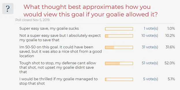
This goal sparked much debate on HFBoards, with one user posting a thread with video of the goal, and a poll asking users to approximate their feelings on it. Among 5 reasonable, well-balanced options, over 50% of users opted for an option which included verbatim "not upset my goalie didnt save that."
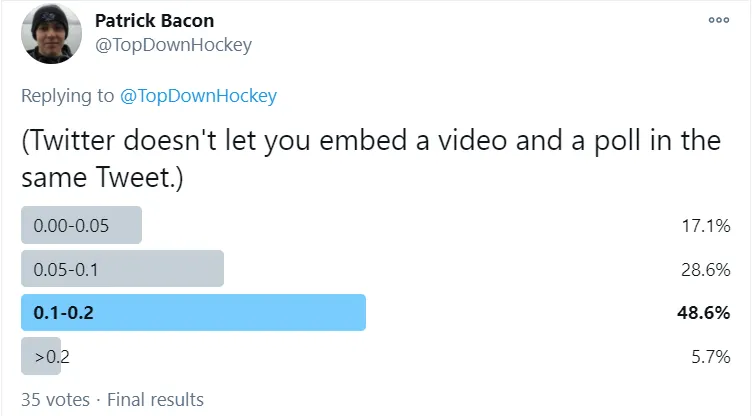
As a Sharks fan who was quite fed up with Martin Jones at the time, I thought the responses were absurd. I was quite upset my goalie didn't save it, and was convinced that people were absolving blame of Jones only because they knew it was a goal. So I took to Twitter, and made a poll of my own, with a deliberately clipped gif that did not show the user the outcome of the shot.

On Twitter, the most popular vote was that the shot had between 10% and 20% goal probability, and nearly half of users had it below 10%.
While the sample size on Twitter is less than ideal, and the two polls were not exactly the same, it's clear enough from this example that fans assign much higher goal probabilities to shots they know are goals, than shots they don't get to see the outcome of.
Training an expected goal model is not that different from training a scout to assign probabilities to goals.
- Just as you give a scout access to features like shot location, everything that happened prior to the shot, and even the announcer's call (by giving them access to video), you give a model access to features like shot distance, angle, etc.
- Just as a scout would give weight to certain features (like "a shot is about 20% more likely if it comes off a royal road pass"), a model gives weight to certain features (like "goal probability is approximately 1% higher every 5 feet closer to the net"). (Note these are both over simplified examples of how weighting works, but illustrate the point.)
- Just as you tune a scout's mindset (like "don't focus on specific, complex patterns until you've seen them at least 30 times"), you can tune a model's hyperparameters. A model with a hyperparameter value of min_child_weight=1 will create a rule from a single example ("that ONE shot from exactly here was a goal, so shots from here are special"), while a model with min_child_weight=30 is more skeptical ("I need 30 similar shots before I believe there's a pattern").
- Just as you train a scout by showing them shots (and which of them become goals, so they recognize which patterns are most dangerous), you train a model by showing it shots and goals and letting it identify patterns.
If we trained a scout by showing them 1,000 shots, and then asked the scout to tell us the probability that one of those shots they saw was a goal, there would be two serious red flags:
- They already know the result, and the probabilities they provide wouldn't be very compelling evidence of whether we actually trained a strong scout.
- They may assign too much value to shots that became goals but weren't actually that dangerous, just like our friends at HFBoards pretty clearly did with Gabriel Bourque's goal. (And conversely, they may assign too little value to really great opportunities where shooters either choked or goalies made heroic saves).
This is why we do not train on the same shots that we evaluate on. The fix for this, in the scout analogy, is simple: Hide some games from the scout and show him the rest, then make him evaluate the shots he hasn't seen the outcome of yet. Then, repeat the process with different games hidden until you've shown the scout all of them. In machine learning, this is essentially what is known as k-fold cross validation.
The part that is a bit more subtle, and where it's easy to accidentally introduce bias, is with hyperparameter tuning. Imagine that you tested 1,000 scouts, each with differing degrees of complexity, and then kept only the results from the scout that gave you the most accurate model. Even without directly showing the scouts the goal outcomes, you'd still be totally cheating, since you'd be choosing the exact best method to "tune" the scout to game the results. Similarly, we can't choose our hyperparameters based on data we see; we need to also choose the hyperparameters for each fold based on a process that is blind to the results.
With this understanding of overfitting in mind, we present our solution: nested cross-validation. We begin by splitting the data into 80 "outer folds" of 41 games each, requiring that all games within each fold come from the same season. (The reason for this will be explained shortly). This creates 32 outer folds of games from 2023-24, 32 for 2024-25, and 32 for 2025-26.
For each of the 80 outer folds: We temporarily remove the outer fold from the dataset and then split the remaining games into 10 "inner folds" in which, once again, require that all games within a fold come from the same season. This generates 4 inner folds with games exclusively from 2023-24, 4 from 2024-25, and 2 from 2025-26. We then randomly generate 100 combinations of hyperparameters to test.
For each of the 10 inner folds: We mark that inner fold as the test set, and the remainder of the inner folds as the train set. We then fit 100 models on the train set (one for each hyperparameter combination) and score each of the models on the test set, and store the results. (By "score" models here, we quite literally mean use those models to assign expected goal values to each shot, and then store those values.)
We then combine the results across each different hyperparameter combinations, i.e., we create 100 different "xG and shots" datasets (one for each hyperparameter combination). We then compute our evaluation metrics across the datasets and select the best one.
Evaluation Metrics
Area Under Curve is the metric that is generally chosen and reported for expected goal models. The metric measures discrimination: How accurately a model is able to discriminate between positive and negative outcomes. (In this case, goals and misses/saves). The University of Nebraska provide a "rough guide for classifying the accuracy of a diagnostic test"
| AUC Range | Classification | Grade |
|---|---|---|
| .90 - 1.00 | Excellent | A |
| .80 - .90 | Good | B |
| .70 - .80 | Fair | C |
| .60 - .70 | Poor | D |
| .50 - .60 | Fail | F |
Rough guide for classifying the accuracy of a diagnostic test. Source: University of Nebraska Medical Center
Unfortunately, discrimination alone is not robust enough to guarantee a good model; it's quite easy to spoof.
To see this in action, we present an extreme example. Imagine we are evaluating 12 shots. 2 are goals, 10 are not. If a model assigns 51% goal probability to the goals and 49% probability to the non-goals, it actually has perfect discrimination, as it accurately identified which of the shots were most dangerous.
Unfortunately, our model would also put out an aggregate value of about 6 expected goals on 2 actual goals. If the model kept that pace over the course of an entire season, with around 7-8 thousand actual goals, this model would easily crack over 20 thousand goals above expected. (!) This model would go a step beyond broken, scorekeeper biased expected goals models of the past that stated Henrik Lundqvist was a better player than Wayne Gretzky, and suddenly say that every goaltender is better than Wayne Gretzky. In spite of perfect discrimination, this model would have poor enough calibration to make it completely useless.
Definition: Calibration
Calibration = xG / goals. For example, if a model assigns 110 expected goals to 100 actual goals, its calibration is 110%.
In order to enforce high calibration, we introduce a new domain-specific evaluation metric: Maximum in-season calibration error.
Definition: Maximum In-Season Calibration Error
This metric measures how far any single season's calibration strays from 100%. For example, if a model achieves 96% calibration in 2023-24, 100% calibration in 2024-25, and 103% calibration in 2025-26, our maximum calibration error would be 4% because 100% - 96% = 4%.
The motivation behind this metric is that aggregate calibration over the 3 seasons could be "spoofed" by a model that under-predicts goal probabilities in one season and over-predicts in another as long as the miscalibrations offset in the aggregate. If a model were 500 goals below expected in 2023-24, perfectly calibrated in 2024-25, and 500 goals above expected in 2025-26, it would be perfectly calibrated in the aggregate, but our metric would identify it being massively overcalibrated for 2025-26, especially considering the season is only halfway through the books.
Our final evaluation metric is area under the curve, under the constraint that our maximum calibration error may not exceed 3%.
Half-Life
Unfortunately, achieving this maximum calibration error proved impossible in our testing when weighting data from all 3 seasons equally. The slightly differing scoring environment of 2025-26, and the fact that 2023-24 and 2024-25 combined have four times as many games of training data as 2025-26, ensure that we significantly over-predict goals in 2025-26. Thus, we introduce a new hyperparameter to weigh seasons differently and improve calibration without discarding seasons entirely: Half-life.
The value of this hyperparameter, which we tune in addition to the standard xgboost parameters (min child weight, max depth, etc.), determines how heavily we down-weigh data from seasons that are far from the season we are currently fitting a model to score values on.
For example, if we are fitting a model to score on 2025-26, a very high half-life would mean that data from 2023-24 still holds much relevance, while a very low half-life would mean we place almost no weight on data from 2023-24. The table below shows this in action with a few concrete examples.
| Source Season | Distance | HL = n | HL = 1 | HL = 2 |
|---|---|---|---|---|
| 2025-26 | 0 | 0.50/n | 1.000 | 1.000 |
| 2024-25 | 1 | 0.51/n | 0.500 | 0.707 |
| 2023-24 | 2 | 0.52/n | 0.250 | 0.500 |
Example: Fitting a model to score 2025-26 shots. Weight = 0.5^(distance / half-life).
To get a better idea of this, let's return to our scouting analogy for a moment. Imagine one scout has trained their brain's expected goal model on 3 seasons of data. They've seen tens of thousands of additional shots from previous seasons, and have learned to identify patterns well enough to accurately rank shots from most to least dangerous. (This is what Area Under Curve measures). But if the NHL's tracking systems or the game of hockey (or both) fundamentally change in different seasons (e.g. goaltenders get better, shots in tight tend to have less pre-shot movement on average, etc.) the scout may systematically over-predict or under-predict goal probabilities depending on the season.
By introducing a half life, we are effectively telling a scout to focus a bit more closely on what they remember seeing recently happen, and discounting some of their older memories. This will slightly harm their pattern recognition and ability to compare shots to one another (lower AUC), but it will ensure that their overall probability estimates will better reflect current conditions (better calibration).
Note 1: This half-life parameter is the reason for our complex, season-stratified architecture. We stratify each fold by season so that each model we fit, both at the outer-fold and inner-fold level, is designed only to score on only one specific season. This way, we are able to properly test the performance of different half-life parameters to identify the best ones, and to actually apply them as well.
Note 2: We applied the half-life parameter only for even strength and power play shots. The small sample size for both shorthanded shots and empty net shots meant that calibration error would not make a significant difference in our overall metrics, and the additional complexity was not worth implementing.
Note 3: If our evaluation metric were unconstrained area under curve, we would likely choose very high half-life values. It is the constraint that forces us to choose from only hyperparameter sets which achieved max calibration errors that fell within our scope.
Formal Procedure
For those who prefer a more precise description, here is pseudocode for our nested CV procedure:
Split data into 20 folds, 164 games each.
    (8 folds with games exclusively from 2023-24, 8 from 2024-25, 4 from 2025-26)

For outer fold i in {1, ..., 20}:
    • Hold i out from dataset.
    • Split remaining games from folds {1, ..., 20} \ i into 10 inner folds.
        (4 folds with games exclusively from 2023-24, 4 from 2024-25, 2 from 2025-26)
    • Randomly generate n combinations of model hyperparameters,
        one of which is season-weighting half-life.
    • For inner fold j in {1, ..., 10}:
        ◦ Mark j as the test set and inner folds {1, ..., 10} \ j as the train set.
        ◦ Fit n models on the train set, score each on the test set, and store the results.
    • Aggregate results by hyperparameter set.
    • The best hyperparameter set in the aggregate, according to our eval metric
        over the 10 inner folds, is the winner.
    • Fit the model on all 10 inner folds using these winning hyperparameters
        and score on the outer fold. These are the final, backfilled xG for that outer fold.
Ongoing Model Updates (Technical Note)
The procedure above describes how we backfilled the data for 2023-24, 2024-25, and the first half of 2025-26. For the second half of the 2025-26 season, we will simply split the entire dataset into 10 inner folds, identify a set of optimal hyperparameters for those 10 folds using cross validation, and fit a model on this entire sample using the optimal hyperparameters we identified. This model that we fit will be our expected goals model going forward that we use to score shots during the remainder of the 2025-26 season. (This is effectively the same process we implemented for each outer fold during the backfill, we're just not holding out any outer fold during this final fitting.)
At the end of the 2025-26 season, we will re-visit the nested CV approach, re-doing the backfill of the entire sample size with data from 24 outer folds (8 from each season), and then fitting our 2026-2027 Expected Goals Model on the entire sample size of 2023-24 through 2025-26. As such, the backfilled expected goals values for the current sample of the 2023-24 season through the first half of the 2025-26 season will change slightly once more at the end of this 2025-26 season, as they will be computed on models that have also seen the second half of the 2025-26 season (which has yet to be played).
Results
Our new model boasts considerable improvement over previous iterations:
- Our models at even strength officially achieve "good" results for AUC (0.8) over the pooled 3-year sample, and are extremely close to good at all situations.
- Calibration at all situations meets the requirement we enforced out-of-sample during the tuning process.
- For the first half of 2025-26, we are at 82 goals above expected; much less concerning than our previous mark of 332, and a number that we can reasonably interpret as "goalies are playing extra well this season."
We now dive into the full results.
Overall Performance
| Strength | xG | Goals | Calibration | AUC |
|---|---|---|---|---|
| Even Strength | 13,786.7 | 13,798 | 99.9% | 0.800 |
| Power Play | 4,438.8 | 4,425 | 100.3% | 0.695 |
| Shorthanded | 474.1 | 468 | 101.3% | 0.796 |
| Empty Net | 1,212.2 | 1,205 | 100.6% | 0.739 |
| All Situations | 19,911.7 | 19,896 | 100.1% | 0.796 |
Per-Season Breakdown
| Strength | Season | xG | Goals | Calibration | AUC |
|---|---|---|---|---|---|
| Even Strength | 2023-24 | 5,470.7 | 5,584 | 98.0% | 0.802 |
| 2024-25 | 5,503.2 | 5,458 | 100.8% | 0.801 | |
| 2025-26 | 2,812.9 | 2,756 | 102.1% | 0.794 | |
| Power Play | 2023-24 | 1,830.6 | 1,821 | 100.5% | 0.699 |
| 2024-25 | 1,700.6 | 1,713 | 99.3% | 0.698 | |
| 2025-26 | 907.6 | 891 | 101.9% | 0.679 | |
| Shorthanded | 2023-24 | 209.1 | 207 | 101.0% | 0.822 |
| 2024-25 | 179.3 | 179 | 100.1% | 0.787 | |
| 2025-26 | 85.7 | 82 | 104.5% | 0.738 | |
| Empty Net | 2023-24 | 444.6 | 443 | 100.4% | 0.710 |
| 2024-25 | 520.5 | 520 | 100.1% | 0.752 | |
| 2025-26 | 247.0 | 242 | 102.1% | 0.754 | |
| All Situations | 2023-24 | 7,955.0 | 8,055 | 98.8% | 0.797 |
| 2024-25 | 7,903.6 | 7,870 | 100.4% | 0.799 | |
| 2025-26 | 4,053.2 | 3,971 | 102.1% | 0.786 |
Comparison to Previous Model
The table below compares aggregate metrics from our original expected goals model (evaluated on 2018-2021) against our new model (evaluated on 2023-2026).
| Strength | Previous Model (2018-2021) | New Model (2023-2026) | AUC Δ | ||
|---|---|---|---|---|---|
| AUC | Calib | AUC | Calib | ||
| Even Strength | 0.777 | 98.8% | 0.800 | 99.9% | +2.3 |
| Power Play | 0.691 | 99.6% | 0.695 | 100.2% | +0.4 |
| Shorthanded | 0.809 | 101.4% | 0.796 | 101.5% | -1.3 |
| All Situations | 0.759 | 99.0% | 0.796 | 100.1% | +3.7 |
* We compared 2018-21 to 2023-26 for an unequivocal comparison between data from before and after the reported tracking changes.
Our expected goal models were previously fair (0.7-0.8 AUC) at even strength and all situations, and closer to good than bad. They are now "good" at even strength in the pooled sample, "good" at all situations in 2024-25, and are a rounding error away from being "good" at all situations in the pooled sample. It is very possible that when we re-train our model at the end of the 2025-26 season to incorporate the remaining data from games that haven't been played, we will have our first "good" public expected goals model at all situations.
These results are due to a combination of improvement in model architecture (primarily the new features we've added, which help proxy for pre-shot movement), as well as more accurate event location data. We thank the NHL for their ongoing efforts to improve the accuracy of the data that they provide to fans and analysts.
Conclusion
The structure of the data the NHL reports is continuously changing, even years after their official big roll out of new tracking technology. It also appears that NHL play styles are legitimately changing as well to some degree. Models that haven't adapted to these changes are at best leaving improved accuracy on the table (as ours certainly was), and at worst fundamentally broken (as ours arguably was).
Fortunately, these changes have also provided more granular and accurate data, which have allowed us to improve our models significantly and nearly reach "good" status at even strength and all situations. (Power play is still "poor" but is very close to "fair").
Because expected goals are now more accurate, downstream player evaluation metrics like GSAx are now also more accurate. Private models remain superior to public models, but the discrepancy between them now has more to do with private data incorporating extra information like pre-shot and player movement, rather than public data just being less accurate in terms of location.
The NHL's tracking systems will continue to evolve, and the game itself will continue to change. At Hockey Stats, we will adapt accordingly.
Explore Our Data
See our new xG model in action with live goalie stats and player evaluations.
Looking for our previous xG methodology (2018-2022)? View the legacy article