At the 2013 NHL Entry Draft, the San Jose Sharks traded the 20th and 58th overall selections in said draft to the Detroit Red Wings in exchange for the 18th. San Jose would go on to select Mirco Mueller with the 18th, while Detroit would select Anthony Mantha with the 20th and Tyler Bertuzzi with the 58th.
I don't have psychic vision, so I had no idea that Mantha and Bertuzzi would both become very good NHL players, or even that both would be available with the picks San Jose surrendered. But as a Sharks fan, I still hated this entire ordeal from the moment it happened. The trade itself was a blatant overpayment, as the 58th pick is far more valuable than the gap between 18th and 20th. But I couldn't even focus on the trade because I was so unhappy with the selection we made.
Mirco Mueller was fresh off a draft year which saw him score 31 points in 63 games with the Everett Silvertips of the Western Hockey League, good for a points per game (P/GP) of 0.49. I had never actually seen him play, but I knew that greatness seldom came of defensemen who scored less than half a point per game in the Canadian Hockey League (CHL) in their draft year, and I didn't think it was wise to spend a 1st round pick in the hopes that he would buck the trend.
Eight years later, I'm mostly vindicated. To Mueller's credit, he's not a complete bust; he's played in 185 NHL games and provided just over 1 Win Above Replacement (WAR) according to my model. But he's also 26 years old, he also spent the entirety of the 2020–2021 season in Sweden, and he's also signed up to spend the entirety of 2021–2022 in Switzerland. His NHL career is almost certainly done, and he hasn't even played 200 games. This pick wasn't the worst of all time, but the final verdict is clear: Selecting Mirco Mueller with the 18th overall pick was not a success.
Why Points Matter Outside the NHL
Those familiar with me may be surprised to hear that I used to care all that much about how many points a defenseman scored in any league. They may be even more surprised to know that I still care. If I've consistently advised against using points to evaluate NHL defensemen, and even gone on record saying that I don't consider Tyson Barrie — the NHL's leading scorer among them in 2021 — a good defensemen, then why do I care about points scored by defensemen outside the NHL? The answer is two-fold:
- I care about the best thing we have. The NHL provides the public with a wide array of information that can be used to build metrics that are far more valuable than points, both for the purpose of describing past performance, and the purpose of predicting future performance — especially for defensemen. Most other leagues don't.
- I hold an underlying assumption that in order for defensemen (and forwards) to succeed at either end of the ice in the NHL, they need some mix of offensive instincts and puck skills that's enough for them to score at a certain rate against lesser competition.
Reason one is straight forward and tough to argue against. In my latest article, I not only documented updates made to my Expected Goals and WAR models, but also performed a few tests to validate whether WAR is superior to points for the purpose of evaluating NHL skaters from a descriptive and predictive standpoint.
If you haven't read it already, I suggest you do so. But I also understand if you don't want to, in which case the results below are still enough to show the superiority of WAR to skater points as a descriptive metric:
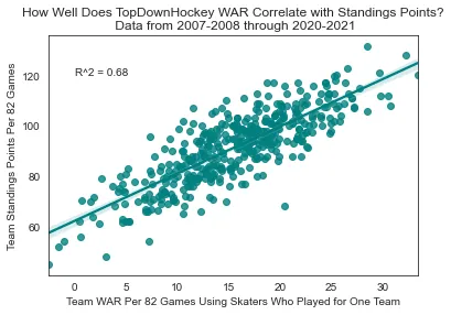
Team WAR correlation with standings points (R² = 0.68)
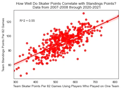
Team skater points correlation with standings points (R² = 0.55)
On the predictive side of things, these test results also display the superiority of WAR:
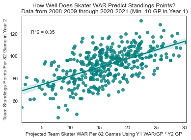
Skater WAR → Standings (R² = 0.35)
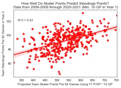
Skater Points → Standings (R² = 0.23)
These tests also validated was that points are not completely useless, or even that much worse than WAR. In the absence of WAR or a similar metric, points are far more useful than nothing. They're actually even more useful at the NHL level than I thought they were when I initially went into this project.
The Research Project
Reason two is a bit more dicey. It's an assumption I made after reading some fairly rudimentary analysis back in 2013, and one I've since used confirmation bias from Mirco Mueller's career to hold on to. The analysis which spawned this assumption is also not unlike the majority of draft research I've read in that it uses games played at the NHL level as the measure of success. Games played are far from a robust or accurate measurement of a player's contribution to their team, and I'd argue that selection bias makes them even worse than points.
Either way, both metrics have their flaws, and two months ago I decided the time was long overdue for me to challenge my pre-conceived notions and determine just how well scoring outside the NHL can predict a player's true contributions at the NHL level. I did so with a two-step research project:
- Build an NHL Equivalency model in order to determine the value of a point in over 100 different leagues that feed the NHL (either directly or indirectly).
- Build a predictive model that uses a player's NHL Equivalency and various other factors such as height, weight, and age to determine the likelihood that a player will become an above replacement level player and/or a star in the NHL according to my WAR model.
In part 2 of this series, I document the process of building the NHL Equivalency Model.
Part 2: Building the NHL Equivalency Model
In Part 1 of NHL Equivalency and Prospect Projection Models, I made a few references to scoring outside the NHL. This would be an easy thing to measure if all prospects played in the same league. It would even be fine if they all played in a small handful of leagues that were similar enough to compare players in each of them, like the 3 leagues which make up the CHL. The analysis I referenced earlier compared scoring from defensemen in all 3 CHL leagues and treated those scoring rates as equal, and I didn't have much of a problem with that because they're all fairly similar.
Not all prospects come from the CHL or a directly comparable league, though. Take Tomas Hertl, San Jose's 1st round selection one year prior to Mirco Mueller, as an example: Hertl spent the entirety of his draft year in the Czech Extraliga, the top men's league in the Czech Republic, and scored 25 points in 38 games (0.66 P/GP). A forward who scored at that rate in any of the CHL leagues in their draft year might be in danger of being skipped entirely in the draft, or at least waiting until a later round to hear their name called. But Hertl was selected 17th overall. And unlike Mueller, selecting Hertl has made San Jose look very smart; his NHL career performance ranks 2nd in WAR and 3rd in points among his draft class, and he would certainly go much higher than 17th in a re-draft.
Hertl's high draft selection and subsequent success at the NHL level shouldn't come as a surprise to anybody because his scoring rate in his draft year was actually better than that of anybody else in his draft cohort. His raw point rates just didn't reflect it because he played in a league where it was significantly tougher to score.
How do I know that Hertl played in a league where it was tougher to score? Just the fact that he played against grown men instead of teenagers isn't enough to confirm this. After all, my beer league is full of grown men, but a team full of the worst teenagers in the OHL would still light our best team up if they went head-to-head. And while common sense may be enough to tell us that the Czech Extraliga is better than any CHL League, and that Hertl's draft year scoring is better than that of a CHL forward who scored at the exact same rate, we can't accurately say how much better it was, or compare to it to players who scored at different rates in other leagues without a measurement of how much good the Czech Extraliga and those other leagues are.
This underscores the need for an equivalency model: One which determines the value of a point in any given league around the world. I built mine out as an NHL Equivalency (NHLe) model on the scale of 1 NHL point, which means that if a league has an NHLe value of 0.5, one point in that league is worth 0.5 NHL points.
Classic NHLe Methodology
A "classic" NHLe model calculates the value of a point in one league by directly comparing how a set of players scored in one league to how those same players scored in the NHL, typically in the same year or the year immediately after. In "League Equivalencies," one of the earliest published works on this subject, Gabriel Desjardins laid out his method:
To determine the quality of the AHL (or any other league), we can simply look at every player who spent year one in a minor league and year two in the NHL and compare their PPG averages. In other words, the league quality relative to the NHL is:
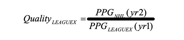
Image from League Equivalencies by Gabriel Desjardins
This methodology is very effective in its own right, but suffers from three issues:
- The development which players undergo between year 1 and year 2 is effectively "baked in" to the model, which skews it in favor of leagues with younger players. If League A is exactly equal to League B in every manner except that League A is full of younger players, then it stands to reason that NHL imports from League A will undergo more development in between years 1 and 2 than those from League B, and thus, score more in year 2. This will lead the model to erroneously state that League A is more difficult to score in, when it really just has younger players who develop more before they see the NHL.
- Using the average points per game in each league makes the data more susceptible to being skewed by extreme values and does not take sample size into account. A player who plays only one game in league A and one game in the NHL holds the same weight as a player who plays 82 games in both.
- This method only works for leagues that directly produce NHLers in the following season. It is impossible to use this method to calculate an NHLe value for a league like the GTHL U16 where players literally cannot play in the NHL in the following season. In addition, while a handful of leagues do produce NHLers in the following season, many of them produce such a small amount that one outlier in either direction can heavily throw off the final estimate.
Network NHLe: The Solution
All three of these problems were remedied in one place when CJ Turtoro published Network NHLe, an excellent piece which I recommend you read. (As a side note, I cannot thank CJ enough for all the effort he put into publishing his initial work and the help he provided me with mine. People like CJ who not only possess the intelligence and domain knowledge to help others, but also the kindness and genuine passion required to do so, are what make the hockey analytics community an unstoppable army of nerds becoming wrong less frequently.)
CJ handled the first problem by using only transitions between players who played in two leagues in the same year. (I also did this and never seriously considered using multi-year transitions.)
He handled the second problem by dividing the total sum of points in a league by the total sum of games played.
The third problem — which I consider the biggest of the three — he handled with a network approach, using indirect paths between leagues to determine the relative strength of each of them. The following example uses fictional data with nice round numbers to explain how one indirect path is calculated:
- 100 players have played in League A and League B in the same year. They scored a total of 1,000 points in 1,000 games in League A (1.0 P/GP) and 500 points in 1,000 games in League B (0.5 P/GP). In order to determine the "League B Equivalency" of League A, we divide points per game in League B by points per game in League A, which works out to 0.5/1.0 = 0.5.
- 500 players have played in League B and the NHL in the same year. They scored a total of 1,000 points in 1,000 games in League B (1.0 P/GP) and 200 points in 1000 games in the NHL (0.2 P/GP). We follow the same methodology laid out above to calculate the NHL equivalency of League B: 0.2/1.0 = 0.2.
- We know that League A has a "League B Equivalency" of 0.5 and League B has an NHL Equivalency of 0.2. In order to determine the NHL Equivalency of League A, we simply multiply these two values by one another: 0.5*0.2 = 0.1. This path states that a point in League A is worth 0.1 NHL points.
No players need to have ever played in League A and the NHL in the same season for this methodology to work. So long as there is a connecting league in between the two, an NHLe value can be calculated for League A.
Real-World Path Examples
Here's an example of a real path that starts with the KHL and uses the AHL as a connector:

KHL → AHL → NHL path example
In this case, players who played in the KHL and the AHL in the same year scored at an aggregate rate that was 1.63 times higher in the AHL than the KHL. This means the "AHL equivalency" factor for the KHL here would be 1.63. Meanwhile, AHL players who played in the NHL in the same year scored at a rate in the NHL that was 0.38 times the rate they scored at in the AHL. Multiplying these two values together provides us with a value of 0.63, which is the "NHLe" for the KHL for this particular path.
Not all paths feature exactly one connecting league, though. Some paths feature none, and are still completely valid, such as the path of the KHL directly to the NHL:

KHL → NHL direct path
Some, like the path from J18 Allsvenskan to the NHL, feature more than one connecting league:

J18 Allsvenskan → Division-1 → SHL → NHL path
The methodology for leagues with more than one connector remains the same: Calculate the conversion factor for each one league to the next and then multiply the values by one another. In this case, the conversion factor between J18 Allsvenskan and Division-1 (now known as HockeyEttan) is 0.34, the conversion factor between Division-1 and the SHL is 0.1, and the conversion factor between the SHL and the NHL is 0.33. Multiply these 3 values by performing 0.34*0.1*0.33 = 0.012 and the result states that the value of a point in J18 Allsvenskan is about 0.012 points in the NHL. (Note that these values are rounded, and if you manually perform these calculations by hand with the rounded values you will get a slightly different result.)
Selecting and Weighting Paths
What I've shown so far is just the methodology for calculating one path. But unlike classic NHLe, where the only path is the single one with zero connectors, Network NHLe can have dozens if not hundreds of paths! This raises more questions:
- How do we determine the top path to use?
- Once we determine the top path, should we use only that one, or should we use more than one? If more, then how many?
- Are all paths valid, or should we exclude paths with a negligible sample size of transitioning players?
- Do we place different weights on different equivalency scores that we get from each path, or do we just average them all?
The answers to (some of) these questions are where my NHLe differs from Turtoro's, who provided the following answers to each of them:
- The top path will be that with the fewest connecting leagues (he refers to them as edges).
- Roughly the top 5 paths will be used.
- A path must feature at least 10 instances of transitioning players to be valid.
- Paths are weighted by the following formula:Where Connections is the number of connections (including the final connection to the NHL) which make up a path, and MinimumInstances is the minimum number of transitioning players which make up an instance within the path.
Weight = 1/2^(Connections) * MinimumInstances
The might look a bit tricky, so here's an example of three paths being weighted for the KHL:

KHL path weighting example
The first path here is KHL→AHL→NHL. This path has 2 connections. The KHL→AHL connection has 65 instances of a transition and the AHL→NHL connection has 2,876. This means the fewest instances in any connection for this path is 65, and calculation for the weight of this path is 1/2^(2) * 65 = 16.25 .
The second path is KHL→ NHL. This path has one connection with 26 instances of a transition, and the calculation is 1/2^(1) * 26 = 13 .
The third path is KHL→Belarus→WJC-20→NHL. This path has three connections. The KHL→Belarus connection has 130 instances, the Belarus→WJC-20 connection has 75, and the WJC-20→NHL connection has 56, which means the minimum instances for this path is 56. The calculation for the weight of this path is 1/2^(3) * 56 = 7 .
With NHLe values and weights for each path, the process for calculating the league's final value becomes quite simple: Multiply each NHLe value by the weight of its path, take the sum of those outputs, and then divide them by the sum of the weights. In this case, the calculation is ((0.63*16.25)+(0.83*13)+(0.85*7))/(16.25 + 13 + 7) = 26.98/36.25 = 0.74 . If we were to use only these 3 paths, the final NHLe for the KHL would be 0.74.
Parameter Testing and Optimization
I think every answer which CJ provided to these questions is backed by solid rationale. I might have answered these problems differently if I were starting from scratch, but my goal here wasn't just to copy CJ's process and make a few arbitrary decisions to change something I didn't like. My goal was to put together a set of potential answers to these questions that all made sense to me, and then test each of these answers against one another and CJ's, in the hopes of determining an optimal set of modeling parameters for building a Network NHLe model. Here are the different sets of parameters that I decided to test as an answer to each question:
For determining the top path(s):
- Select the path which would have the highest weight according to the weighting equation laid out above.
- Select the path with the fewest connecting leagues, using the highest weight according to the weighting equation as a tiebreaker.
- Select the path with the highest minimum number of instances among all connections.
For determining the number of path(s) to use:
- Test selecting only the single best path through selecting up to the top 15 best paths.
For excluding paths based on sample size:
- Test selecting paths with a minimum of 1 instance through selecting paths with a minimum of 15 instances.
For weighting each path:
- I simply stuck with CJ's weighting formula here. I briefly tried out a few different methods, but his performed better in preliminary tests and just made too much sense.
Additionally, I chose to test out 3 other parameters:
- Including the U20 and U18 World Junior Championships.
- Changing the method of calculating a conversion factor between two leagues. I tested CJ's method of using the full sum of scoring in each league, Desjardins' method of using the mean of points per game in each league, and my own method (suggested by CJ) of using the median of points per game in each league.
- Dropping the first connecting league in one path before creating a new path for that league. For example, if the KHL→AHL→NHL path is used, all other paths for the KHL from that point on may not use the AHL as the first connection. (The initial implementation of this rule was actually an accident caused by me misinterpreting CJ's methodology, but I wound up keeping it as a test parameter because I thought it may be preferable not to weigh any one direct relationship too heavily for a given league.)
Cross-Validation Methodology
With a set of parameters that I all deemed eligible for building out the final model, it was time to test each of them and determine the best. I decided that the goal of my tests would be to minimize the mean absolute error between predicted points per game and actual points per game for all players who transitioned leagues. Predicted points per game was calculated based on the NHLe value for each league and points per game in the first of two leagues, with the NHLe values being those which were obtained after building the model with a given set of parameters.
I know I just threw a word salad at you, but the test process is actually quite simple; I'll break it down using Melker Karlsson in 2010 as an example:
- In this season, Melker scored 35 points in 27 games (1.3 P/GP) in superelit and 2 points in 36 games in the SHL (0.06 P/GP).
- If the NHLe model obtained from a given set of test parameters stated that the NHLe value for the SHL was 0.53 and the value for superelit was 0.08, then we could obtain the conversion factor from superelit to the SHL by performing 0.08/0.53 = 0.15.
- We would then multiply the conversion factor by his scoring rate in superelit and perform 0.15*1.3 = 0.2 , which would give us his projected scoring rate in the SHL. His actual scoring rate in the SHL was 0.06, and the absolute value of the difference between 0.06 and his projected scoring rate of 0.2 is 0.14, which would be the error obtained for this particular transition.
- We would then repeat this process using his scoring in the SHL to predict his scoring in superelit, performing 0.53/0.08 = 6.625 to obtain the conversion factor from the SHL to superelit, and then performing 6.625 * 0.06 = 0.4 to obtain his predicted scoring rate in superelit.
- Since his actual scoring rate in superelit was 1.3 P/GP, the error between this value and his predicted scoring rate of 0.4 would be 0.9. In conclusion, this one transition would give us two error values: 0.14 and 0.9.
The mean absolute error for a given NHLe model is the average of every error value obtained from players who transitioned leagues.
The dataset which I used to run these tests and build my model was all skaters who had played at least 5 games in any two or more of the 124 leagues I used in any single season from 2005–2006 through 2019–2020, with the exception of 2012–2013. (2012–2013 was removed entirely due to the shift in global quality of competition caused by the NHL lockout.) I couldn't simply train my NHLe model using these sets of parameters on my entire data set once and then test it on the same data, though, as my goal was not to find the exact set of parameters that could best predict what has already happened; my goal was to build out the model that could best predict scoring out-of-sample. The way to train it to do so was to "practice" predicting scoring out-of-sample. I did this by randomly splitting my dataset into fifths and performed 5-fold cross-validation.
5-fold cross-validation may sound daunting, but it's not all that scary. You begin with a training set which consists of 4/5ths of the league pairs in the dataset and a test set which contains the other 1/5th of the player pairs. For every single set of parameters which are fed, the NHLe model is built out on the training set and then tested on the test set. This process is then repeated four more times using the other groups of training sets and test sets, resulting in five different test values for each set of parameters. (Note that none of the test/train sets overlap; every single player pairing appears exactly once in one test set and none of the other four test sets, and that same player pairing appears once in the other 4 train sets for which it does not appear in the corresponding test set.)
Fold 1
Fold 2
Fold 3
Fold 4
Fold 5
Cross-validation for each fold is performed using every single possible set of parameters to build the model out on the training set and test it on the test set. After cross-validation is completed for all 5 folds, the average test value is obtained for each set of parameters. The set of parameters with the best average test value (in this case, the lowest mean absolute error) is considered the optimal set of parameters for building an NHLe model.
Optimal Parameters
The results of my 5-fold cross-validation determined the following set of parameters to be most optimal:
- The top path available will be the one with the fewest edges, with total weight being used as a tiebreaker if two paths have the same number of edges.
- Up to the top 11 paths will be used for a league.
- Paths with a minimum of 8 instances of transitioning players are valid; all others will be discarded.
- The World Juniors (both U18 and U20) will both be used.
- The full sum of points will be divided by the full sum of games played in each league to determine the conversion factor between two leagues.
- The first connecting league will be permanently dropped before any further paths are created.
The average of the mean absolute error across these five folds was 0.33. (I computed R² as well, which was also 0.33, but chose not to use it as a target parameter in training.)
Final NHLe Values
With these parameters set, it was time to build out the model using the entire dataset this time around. These are the equivalency scores for every league for the final NHLe model:
| League | NHLe |
|---|---|
| NHL | 1 |
| KHL | 0.772 |
| Czech | 0.583 |
| SHL | 0.566 |
| NLA | 0.459 |
| Liiga | 0.441 |
| AHL | 0.389 |
| DEL | 0.352 |
| Allsvenskan | 0.351 |
| VHL | 0.328 |
| Slovakia | 0.295 |
| EBEL | 0.269 |
| WJC-20 | 0.269 |
| France | 0.250 |
| Belarus | 0.242 |
| Czech2 | 0.240 |
| EIHL | 0.235 |
| LNAH | 0.232 |
| DEL2 | 0.205 |
| Kazakhstan | 0.201 |
| NCAA | 0.194 |
| Denmark | 0.190 |
| Mestis | 0.178 |
| NLB | 0.176 |
| Italy | 0.176 |
| Norway | 0.173 |
| ECHL | 0.147 |
| OHL | 0.144 |
| MHL | 0.143 |
| USHL | 0.143 |
| WHL | 0.141 |
| Poland | 0.135 |
| WJC-18 | 0.135 |
| Russia3 | 0.135 |
| Usports | 0.125 |
| USDP | 0.121 |
| QMJHL | 0.113 |
| Division-1 | 0.109 |
| Czech3 | 0.104 |
| Erste-Liga | 0.103 |
| Slovakia2 | 0.102 |
| Romania | 0.099 |
| Superelit | 0.091 |
| NAHL | 0.087 |
| Germany3 | 0.085 |
| ALPSHL | 0.084 |
| U20 SM-Liiga | 0.083 |
| BCHL | 0.080 |
| NMHL | 0.076 |
| Czech-U20 | 0.074 |
| AJHL | 0.062 |
| EJHL | 0.060 |
| Czech U19 | 0.059 |
| SwissDiv1 | 0.054 |
| Belarus-Vysshaya | 0.052 |
| SJHL | 0.052 |
| U20-Elit | 0.049 |
| CCHL | 0.048 |
| MJHL | 0.046 |
| USPHL-Premier | 0.046 |
| Slovakia-U20 | 0.044 |
| Russia-U17 | 0.044 |
| USPHL-18U | 0.041 |
| U18 SM-Sarja | 0.040 |
| NAPHL-18U | 0.039 |
| Czech U18 | 0.038 |
| J18 Allsvenskan | 0.038 |
| Division-2 | 0.038 |
| MJAHL | 0.037 |
| QJAAAHL | 0.036 |
| MPHL | 0.035 |
| OJHL | 0.034 |
| HPHL-16U | 0.034 |
| Slovenia | 0.033 |
| Russia-U18 | 0.032 |
| 16U-AAA | 0.031 |
| J18-Elit | 0.029 |
| USHS-Prep | 0.028 |
| QMAAA | 0.028 |
| CISAA | 0.027 |
| Norway2 | 0.027 |
| USPHL-16U | 0.027 |
| GOJHL | 0.027 |
| AYHL-16U | 0.026 |
| Russia-U16 | 0.025 |
| J20-Elit | 0.024 |
| USHS-MN | 0.024 |
| DNL | 0.024 |
| Denmark2 | 0.023 |
| VIJHL | 0.021 |
| NOJHL | 0.021 |
| Slovakia-U18 | 0.020 |
| CAHS | 0.020 |
| AMHL | 0.020 |
| PIJHL | 0.020 |
| KIJHL | 0.020 |
| U17-Elit | 0.018 |
| II-DivisioonA | 0.018 |
| U20-Top | 0.017 |
| BCMML | 0.016 |
| U16 SM-Sarja | 0.015 |
| NSMMHL | 0.015 |
| Czech U16 | 0.014 |
| Denmark-U20 | 0.013 |
| MMHL | 0.013 |
| U16 SM-Sarja-Q | 0.012 |
| GTHL-U16 | 0.012 |
| J20-Div.1 | 0.011 |
| U16-SM | 0.011 |
| U16-ELIT | 0.010 |
| Alliance-U16 | 0.009 |
| GTHL-U18 | 0.008 |
| J18-Div.1 | 0.008 |
| Division-4 | 0.008 |
| QMEAA | 0.007 |
| J20-Div.2 | 0.007 |
| Denmark-U17 | 0.006 |
| U16-Div.1 | 0.005 |
| J18-Div.2 | 0.005 |
| ETAHL U18 | 0.005 |
| AMMHL | 0.005 |
| QBAAA | 0.004 |
| AMBHL | 0.002 |
| U16-Div.2 | 0.002 |
Note that a few of these leagues are merged with other leagues. For example, there was a league known as "Russia" in the EliteProspects database before the KHL came along which was effectively the KHL; I simply merged those two together as the KHL. The same goes for "Russia2" and the VHL and another league or two.
Part 3: Prospect Projection Models
The second step of this project was not unlike the first in that it took heavy inspiration from the established work of one of hockey's top public data scientists: Byron Bader. Bader runs Hockey Prospecting, an NHL-Level Analytics Tool which he describes below in his own words:
Hockey Prospecting standardizes player scoring across the board and uses historical performances to chart how prospects will perform in the NHL.
You're probably familiar with Bader and/or Hockey Prospecting by name, but even if you aren't, you've either been living under a rock or you've seen one of his trademark prospect comparison cards:
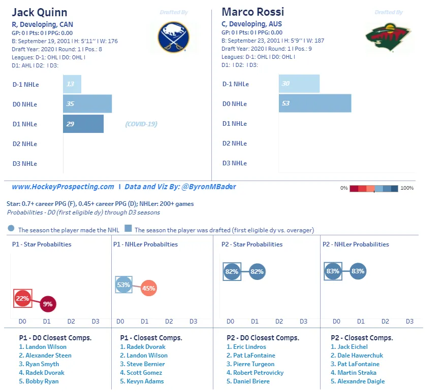
Image from Byron Bader
The essence of Byron's model is that he uses a logistic regression which takes scoring rates to determine the probability that a prospect will become an NHL player and/or an NHL star. A player is considered an NHLer if they play at least 200 games, and they are considered a star if they score at or above a certain rate in their career.
Going into this project, my philosophy for building a prospect model remained very similar to Byron's up until the way I chose define a star at the NHL level, at which point it diverged heavily. As I mentioned earlier, the NHL provides the public with a wide array of information that can be used to build metrics that are more valuable than points, and since my goal here is to use the best information available wherever I can, I chose to use the outputs of my WAR Model to define both target variables.
Defining NHLer and Star
Defining an NHLer
This process was simple: An NHLer is a player who has met the classic criteria of at least 200 NHL games played and provided a positive career WAR. I don't care how many games somebody plays if they aren't adding more than the next player that could be claimed off waivers, so I don't believe any measure of success should be assigned to players who fail to do so.
Defining an NHL Star
This was a slightly more complicated process because star is a completely arbitrary term that varies heavily depending on the context of the discussion, and the textbook definition of star probably has more to do with marketing and exposure than it has to do with how good a player actually is. At the conclusion of the 2019–2020 regular season, Marc-Andre Fleury was a 36 year old in the midst of his second straight mediocre season who had just been relegated to the role of his team's backup for the playoffs. But he was also indisputably a star on the basis of name recognition and jersey sales.
I was obviously not about to define a star using name recognition, as I wanted to use a metric better than points; not a significantly worse one. I knew that I would use my WAR model and use the term "star" strictly as a measure of player quality, but I wasn't sure how to do this until I thought back to some reading I had done some time ago on The Pareto Principle, which you may know as the 80/20 rule.
The Pareto Principle states that 80% of consequences come from 20% of the causes.
In other words, the "vital few" make up only 20% of a given population, yet are responsible for 80% of the outcomes in the population. To give a practical example of this in action, while researching the principle I found a study which showed that the top 15% of MLB baseball players contribute roughly 85% of the WAR. The numbers are not always exactly an 80/20 split, but there generally tends to be a small percentage of the population responsible for an inversely large percentage of the outcomes. My first thought upon reading this was that something similar was also true for my WAR model, but I didn't bother to look any further into it at the time.
When it came time to define a star player, I circled back to the Pareto Principle. I felt that if this principle were true for my model, then the top 15% or 20% of WAR producers — those who would be considered the "vital few" according to the Pareto Principle — would be those considered star players. The more accurate terminology for "the probability of a player becoming a star" in this case is actually "the probability of a player becoming a member of the vital few," but the two are essentially interchangeable, and the term star is much easier to interpret, so I'll stick with it.
I didn't know for sure whether the Pareto Principle was true for my model, and I couldn't just assume it was and use the top 15% figure that was true for the MLB, or use the top 20% figure which Pareto defined.. To determine the Pareto Principle value for a given season, I first ranked all skaters by WAR, then took a number of total skaters (starting with 1) and kept only that number of the top skaters in WAR. I then added the total WAR contributed by those top skaters and divided it by the total WAR added by all skaters in that season. Finally, I took the percentage of the whole body of skaters which they represented and added that to the percentage of the whole body of WAR which their contributions represented. I repeated this process for every possible number of skaters, and determined the optimal value for the Pareto Principle was that for which the sum of the percentage of total skaters made up and the percentage of total WAR contributions from those skaters was closest to being exactly 1.
This may sound like a complicated process — I certainly found it easier to implement than to describe — so take a look at the following example which uses the top-5 potential percentages for 2020–2021:
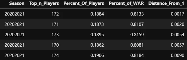
Top-5 potential percentages for 2020–2021
For this particular season, the Pareto Principle was optimized at a point where the top 18.84% of skaters provided 81.33% of the total WAR. Here are the optimal values for every season since 2007–2008:
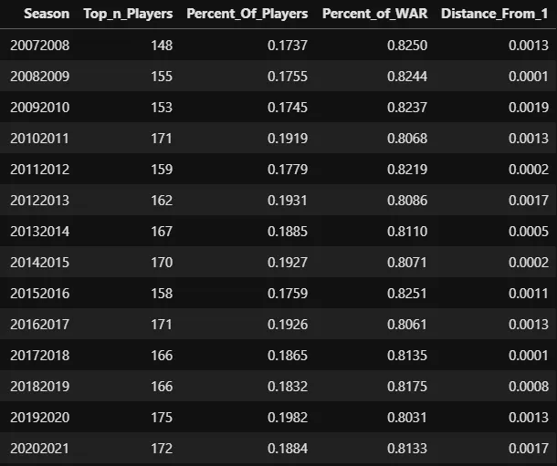
Optimal Pareto values by season
As you can see, the Pareto Principle varies from year to year, and recently it has grown to state that the "vital few" make up a larger percentage of the population than they used to. The gap here is small enough that it could totally just be variance, but my hypothesis is that NHL teams are just doing a better job of optimizing the lower halves of their lineups better than they did back from 2007 through 2010, so the gap between replacement level players and stars is smaller than it used to be. (Note that I already held this assumption, so these results just serve to confirm it.)
After optimizing the Pareto Principle for each season, I determine that the average of the percentage of skaters who make up the vital few across all seasons was roughly 18.5%. I then used this value to form my final definition of a star: A skater in the top 18.5% of career WAR per game rate among all skaters who have played at least 82 NHL games. This worked out to be roughly 1.5 WAR per 82 games played at the career level. This value feels low for a star, and many of the players on the list of established stars are not players to whom I would personally apply that term, but I'm confident enough in the methodology used to define a star that I'm comfortable with the outputs.
Projecting NHLers and Stars
I had a clear definition of what made an NHL player and what made a star. Research has generally shown that hockey players peak from ages 22 through 26 and decline thereafter, so I decided that if a player's D+8 (age 26) season had passed and they hadn't yet established themselves as an NHLer, they would be considered a bust. Those who had yet to be classified as an NHLer, star, or bust were considered "undetermined" and not used in calculating projections.
Once I made this classification, every player who had played their draft season during or after 2006–2007 and either seen their D+8 season pass (even if they were no longer playing hockey at that point) or established themselves as an NHLer and/or star was a data point that could be used to build out the final projection model. Their scoring rates as prospects would work as predictor variables, and their NHL performance (starting in 2007–2008) would be used as target variables.
With a universal measurement of the scoring proficiency demonstrated by prospects alongside the eventual outcomes of these prospects' careers, I had everything I needed to build out the final model: One which leveraged scoring as prospects (as well as a few other less important variables in height, weight, and age) to predict the outcome of a player's career at the NHL level.
Due to the small number of predictor variables in my regression and the fairly simple and predictable way in which I expected them to interact with one another, I determined that logistic regression would be sufficient enough to meet my needs. But one logistic regression model alone is not enough for the following reasons:
- Forwards and defensemen score at vastly different rates as prospects; their scoring rates should only be compared to their positional peers. This raises the need for separate models to be built for forwards and defensemen.
- The probability of making the NHL is not be the same as becoming a star, and different variables may influence these probabilities differently. This raises the need for separate models to be built determining NHLer probability and star probability.
- Prospects find themselves at different stages of development. A player in his Draft-1 season is in a much different position than a player in his Draft+1 season, but I'd like to be able to use all of the information available to determine the likelihood that both players will succeed in the NHL. This raises the need for separate models to be built for players at different stages of their development.
- If one regression model is trained on the same sample that it is used on, it runs the risk of becoming overfit. To give a practical example, a model that already knows Brayden Point became a star in the NHL may use the data point of a player with Brayden Point's profile to overstate the likelihood that he was going to become a star given the information available at the time. This raises the need for separate models trained out-of-sample to be built for each season.
Here is what the process looks like for building out a model for all skaters who played at least 5 games in any one league during their Draft-1 and Draft seasons:
- Remove players whose draft years were 2007 from the training data, then split the training data into forwards and defensemen.
- Use the forwards in the training set to train a logistic regression model which uses Draft-1 year NHLe, Draft year NHLe, height, weight, and age as predictor variables and making the NHL as the target variable.
- Repeat the process with a model that is identical except that it uses becoming an NHL star as the target variable.
- Take the two logistic regression models which were trained on forwards and run the models on forwards whose draft year was 2007.
- Repeat steps 2, 3, and 4 using the defensemen in the training set.
- Repeat steps 1 through 5for all skaters whose draft year was 2008, and so on and so forth for until you reach skaters whose draft year is 2021.
This process was repeated for all players at different stages of their development using whatever information was available, starting with players in their Draft-2 year and working up to players in their Draft+5 year. This means that a model was built which used Draft-2 year NHLe through Draft+5 year NHLe, along with a model for everything in between: Draft year through Draft+5, Draft-1 through Draft+3, etc.
Model Limitations and Considerations
Remember that the end values of my NHLe model can be interpreted as a very simple equation: 1 point in League A is worth X points in the NHL. One downside of this rudimentary equation appears to be the lower ceiling for the NHLe values of players who play in weaker leagues. The fact that hockey games only last 60 minutes and very few players play more than 30 means there is a cap on how much any player in any league is physically capable of scoring.
Take the GTHL-U16, for example: The league has an NHLe conversion rate of 0.012. While any NHL player would completely dominate it, they would also not score anywhere near the 83 points per game necessary in that league to post an NHLe of 82. The Connor McDavid of today, whose NHLe in 2020–2021 was 153.75, would probably struggle to manage an NHLe of even 40 if he were banished to the depths of the GTHL-U16.
While the McDavid fantasy scenario I laid out is extreme, this issue is legitimately present on a lesser scale with prospects who can only dominate junior leagues to such a degree. Even if the NHLe conversion values are accurate for the entirety of the population, the ceiling for the NHLe which high end prospects can post is much lower for those playing in junior leagues than it is for those playing in men's leagues where each point is far more valuable.
In addition to this modeling quirk, it should also be kept in mind that the NHLe model already appears to be quite high on professional men's leagues and relatively low on junior leagues, at least relative to conventional wisdom. Both of these factors mean that the prospect projection model, and especially the star probabilities from the model, are more favorable to European players. This can be seen in the 20 players who had the highest star probability using their Draft-1 and Draft seasons.
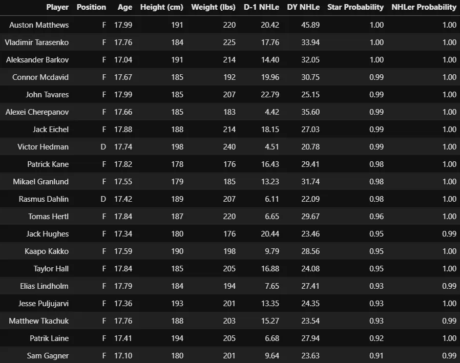
20 players with highest star probability
The list contains a high proportion players who spent their draft year in Europe. While the model did a good job of identifying undervalued players from European leagues in Tomas Hertl and Vladimir Tarasenko who weren't drafted in the second half of the first round, I'd say it was still a bit too confident in those players, and also too confident in players like Mikael Granlund (who just narrowly meets the star cut-off) and players like Kaapo Kakko and Jesse Puljujarvi whose career outcomes are still up in the air.
While the logistic regression itself is trained out-of-sample, it's still not entirely fair to use the outputs of this model as though this information was all available at the time these picks were made because roughly half of the information used to inform the logistic regression for each season actually happened after that season.
For example, the model which says Patrick Kane had a 98% probability of becoming a star and a 100% probability of making the NHL may not have known that a player with Kane's exact profile did both things, but it knew everything else about players from every other draft year from 2008 through 2020. These things had yet to happen in 2007, and the information which stemmed from them was therefore not available. In addition, the NHLe model itself — by far the most important component in these regression models — also suffers from this same issue (and was not even trained out-of-sample).
Model Validation
This is all by way of saying that a comparison between what my model would have suggested NHL teams do on the draft floor and what they actually did would be inherently unfair to those NHL teams, who also undoubtedly would have used this new information to inform their future decisions. Nikita Kucherov's draft year (2012) was two years after Artemi Panarin's, but if NHL teams somehow knew in 2010 that Nikita Kucherov would become one of the greatest players in the world (like my model for 2010 forwards did), they would likely have viewed Artemi Panarin in a different light even if they didn't specifically know his future. Until I can devise a fair way to compare the outputs my model to the draft performance of NHL teams on equal footing, I won't try and do so.
I can, however, still test the performance of my model according to two metrics: Area Under Curve (AUC), which you can read about here, and Log Loss, which you can read about here. The results of these tests are laid out below:
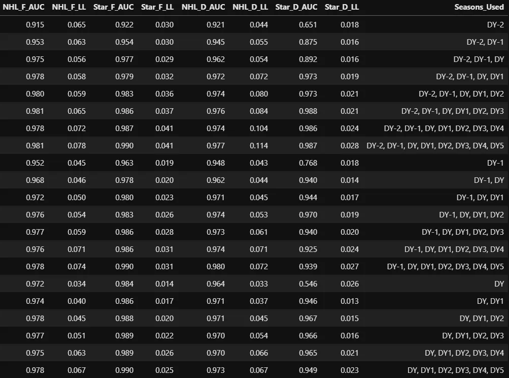
AUC and Log Loss test results
For whatever reason, the star defenseman model struggles to post a strong AUC when provided with only one season of data, regardless of whether that season is the Draft-2, Draft-1, or Draft Year. Outside of that, every single model posts excellent test metrics: The documentation for AUC which I linked above states that a model which scores between 0.9 and 1.0 is excellent, and log loss values below 0.1 are generally considered excellent as well.
None of this necessarily means I built out a great model, though. This is because not only do the vast majority of players in this data set fail to make the NHL — much less become stars — but because they almost all exhibit signs that make their failures extremely easy to predict. Take 2010 as an example, where 2,706 players were eligible to be drafted and used in the model: Of those 2,706 draft-eligible players, only 462 had at least a 1% probability of making the NHL and only 126 had at least a 1% probability of making a star.
While most of these players are irrelevant, it's also fair to say that a model deserves some degree of credit for identifying bad players. At what point should you stop giving that credit, though?
I spent some time pondering over this before eventually deciding that if no NHL team would draft a player, a model shouldn't receive credit for agreeing on such an obvious statement. But I couldn't just exclude all undrafted players, as it would be very unfair to the model to exclude a player like Artemi Panarin, who had a 78% chance of making the NHL and 32% probability of becoming a star based on data from his Draft-1 and Draft Years.
What I chose to do was simply to exclude all players whose NHLe in their Draft-2, Draft-1, or Draft years were below the threshold of any player who had been drafted in any year. This unfortunately didn't actually change much, because players with an NHLe of 0 in their Draft-2 year and Draft-1 year have been drafted, and players with an NHLe below 1 in their Draft year have been drafted. The test results for the performance of the model on only "draftable" players is essentially identical, and for some sets of seasons where the minimum NHLe is 0, they are exactly identical.
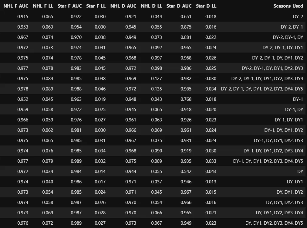
Model performance on draftable players only
As you can see, the model still performs mostly excellent according to these test metrics. The only area where it struggles even slightly is with predicting star defensemen early in their career, which brings me back to the assumption I made in part 1 of this article:
In order for defensemen (and forwards) to succeed at either end of the ice in the NHL, they need some mix of offensive instincts and puck skills that's enough for them to score at a certain rate against lesser competition.
As it turns out, the hardest thing for scoring rates as a prospect to predict is whether a defenseman will become an NHL star; the model does a fair, but not necessarily good or great job predicting this alone with only one year of data. With multiple years of data, though, the model does a very good job of predicting star defensemen.
Conclusion
In closing, I would say that my research mostly confirms the assumption I made: The rate at which a defenseman scores as a prospect is very important, and I greatly recommend against using high draft picks on defensemen who aren't proficient scorers.
This concludes part 3 of the series, and the documentation for the model. Chances are that if you've already read through the ten thousand or so words I've written so far, you've got some kind of interest in the 2021 draft. If that's the case, then I have good news for you: This series has a part 4 which will break this draft class down in detail!